Statistics for decision

La notion d'écart-type est déjà abordée dans la partie probabilités. Ce chapitre a pour objectif de montrer pourquoi cette notion a été introduite. Pour cela, considérons les deux populations suivantes avec les différentes notes dans deux groupes différents.

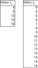
When we compute the mean for group1 and for group 2, we find the same result, 10. This forces us to push our description beyond the mere central tendency to characterise more precisely our populations.

The objective of the variance is to quantify another characteristic of the population: its homogeneity.

Considering group 1 and 2, which one is the most homogenous?

The answer, intuitively, is group 2. But how shall we quantify this compelling vision?

First of all, the range of grades within the set did give us a hint as to the right answer, the range is 12 for group 1 and 8 for group 2.

Yet, soon enough, we realise that this method would be quite misleading in a number of cases, suffice to imagine the following distribution of grades:

Notes (sur 20) groupe 3

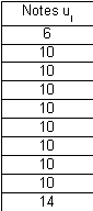
Here, the mean is 10, and the range 12, so why do we keep suspecting that group 3 is more homogenous than group 2 ?

Of course, for the sake of robustness, the evaluation of homogeneity must take into account all the individuals forming the set, looking only at the extremes is futile.

As we remember that the mean represents a kind of central point for the distribution, it seems interesting to look at how “far away” from the center each member of the population is, this is simply the difference between each x_i and the mean .

If we sum those differences we get closer to a measure of homogeneity.

But the method is flawed, since some of the differences will be positive and some will be negative, a good portion of the terms will cancel out, leaving a meaningless number for us to examine. Indeed, in our example .

In order to force the differences into positive territory we are tempted to introduce the sum of the absolute value of the differences i.e. .

Unfortunately, the absolute value brings on-board a number of predicaments (including but not limited to non-differentiability).

Ultimately, we resort to squaring the differences, which also guarantees positive values. The calculation applied to group 1 and 2 shows and .

This would indicate that group 1 is more homogenous than group 2, which was contrary to our keen initial scrutiny.

This issue comes from the number of individuals in each population, in order to compare, we shall use the mean of the squared differences between the grades and the mean of the grades, or .

This value is called variance with the notation V(x).

In the example, we find 24.5 as the variance for group 1and 10.4 as the variance for group 2.

Thus, we conclude: the larger the variance, the lower the homogeneity.

Finally, the order of magnitude of the variance is not significant since we squared the differences (the “distances”, although positive, were distorted).

In brief, we have the following formula:

V(X)=

For the sake of easy calculation, we will use an equivalent formula:

Indeed :

We are highly satisfied with our quantification of the homogeneity and the variance formula. However, we did mention that the choice of squared values, while indispensable, was distorting the numerical result. Besides, if we are dealing with an “age” variable in years for example, the variance's unit will be years², a non-intuitive notion to manipulate (for your boss).

We are now looking for an order of magnitude closer to the reality of the dataset.

Therefore we decide to use the square root of the variance, with the notation σ, where σ =.

We find respectively 4.95 and 3.22 as the standard deviations of groups 1 and 2.

Under this form, we are happy to simply explain that the grades are, on average, at a distance of 4.95 points away from the mean of group 2 (i.e. 10).

Let us now show the table that helped us calculate the standard deviation.

Ecart type du groupe 2

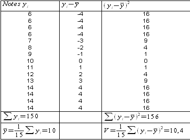
So σ =.

In this chapter, we studied the variance and standard deviation for discrete series.

For continuous series, the method is identical, with preparatory step of choosing a specific value for each class, namely the center of the class.