
Known distributions (normal distribution, Student distribution, ...)
After studying various characteristics of a quantitative variable (mean, median, quartile, standard deviation,...) we can try and associate such variable with laws defined in probabilities theory. This paragraph reviews or details the behaviour of some classical laws often used in statistics.
It is unnecessary to know all the laws' formulae, yet your duty is to know how to use them.
The only definition to commit to memory (and understanding) is that of the density.
Définition : Density
A real-valued random variable X has a density function p, if there is a real- valued function such that:
![]()
meaning that the probability P for this variable to lie between a and b is equal to the integral value of the density p.
The notion of density is very convenient to graphically understand the behaviour of a variable, as we shall see in the famous example of the bell curve (also called Gauss or Gauss-Laplace curve).
Normal distribution (or Gaussian distribution, bell curve distribution...)
This is a very common law, frequently observed in nature. E.g. the height of the human population follows a normal distribution: many individuals have a height close to the mean height of the population and few individuals are either very short or very tall.
A variable U follows a standard normal distribution if its density on real line ![]() is defined as:
is defined as:
![]()
If μ is a real number and σ a positive real number, the Gaussian distribution, or normal distribution N (μ, σ) of the density on ![]() is defined as:
is defined as:
![]()
In such case, we note that μ is the mean (also called expectation), and σ the standard deviation.
As far as calculation is concerned, we resort to tables.
Let us have a random variable X, following a normal distribution N (μ ,σ). We may find an interest in calculating the probability for X to have a value belonging to the interval [a,b] (it could be the income range of the people you target as a sales person, or the range of shoe sizes you plan to keep on stock).
Thus, ![]() .
.
In order to calculate this integral, we introduce the variable ![]() .
.
The integral becomes ![]()
with ![]() .
.
We realise the density obtained after the change of variable is that of the standard normal distribution.
Therefore, if we define U as a random variable such that ![]() , U follows a standard normal distribution N (0 ,1) and
, U follows a standard normal distribution N (0 ,1) and
![]() .
.
But these integral calculations are not always straightforward ( we strongly advise against trying to find a primitive to the Gaussian density). To solve such calculation, we use standard normal distribution tables displaying results for pre-set values.
We now understand the necessity to standardise the distribution (i.e. to consider the U variable rather than the X variable), since it is impossible to pre-calculate tables for every possible parameter (μ ,σ).
E.g. tables provide values for the cumulative distribution function ![]() of the random variable U following a standard normal distribution (@@@INSERER référence à la table ), meaning the function :
of the random variable U following a standard normal distribution (@@@INSERER référence à la table ), meaning the function :
![]() .
.
This function has the following properties :
![]() (−u) = 1 −
(−u) = 1 −![]() (u)
(u)
![]() (0]=0,5
(0]=0,5
as a consequence ![]() .
.
Refer to the table link here to find out how to read it and make calculations.
Another interesting activity is to express the deviation of the X variable from the mean as a multiple of the standard deviation σ.
Let us try and compute, for k>0 :
![]() .
.
It is important to remember a remarkable value in the tables: P (−1, 96 < U < 1, 96) = 0, 95. The value 1.96 is important because if we decide to say: “The variable U belongs to the interval [-1.96; 1.96]”, we know we take a risk of 5% to be wrong.
Similarly, with a risk of 1% of error, U belongs to the interval [-2.576; 2.576].
There are also tables to find these 1.96 and 2.576 figures, they are called fractiles tables.
We use the notation ![]() for the fractile of order
for the fractile of order ![]() , i.e. the number such that
, i.e. the number such that
![]() .
.
The fractiles provide invaluable information.
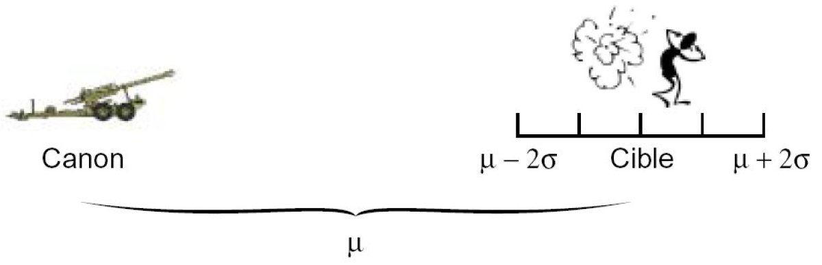
Let us imagine the range X of a TRF1 artillery canon follows a normal distribution with the parameters μ =24km and σ=25m
Proposition 1.10 let X be a random variable following a normal distribution N (μ ,σ), we have :
P (μ − 1, 96σ < X < μ+ 1, 96σ) = 0, 95.
We can then say that 95% of the shells will fall in a zone between 24km-50m and 24km+50m.
If we wish to find the zone where 99% of the shells will fall, we use the fractile of order 0.995, the table gives a value of 2.57.
We get P (μ − 2, 57σ < X < μ+ 2, 57σ) = 0, 99 and conclude that 99% of the shells will fall in a zone between 24km-65m and 24km+65m.
This demonstrate the huge benefits we get if we can demonstrate that a variable follows a normal distribution. For this there are normality tests, that allow us to use or reject the hypothesis that a random variable follows a normal distribution.
Chi-squared distribution
Let us consider ν independent, random variables U1, U2, · · ·, Uv, each following a standard normal distribution N (0 ,1). We will name Chi-squared distribution with ν degrees of freedom the distribution followed by the variable ![]() . We shall use the notation
. We shall use the notation ![]() for this distribution law.
for this distribution law.
Its density function is defined as:
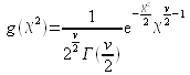 .
.
Its mean (or mathematical expectation) is ν, and its variance is 2 ν.
As for the normal distribution, we shall use the tables linked here (@@@@INSERER REFERENCE).
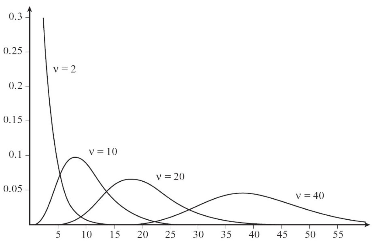
Student distribution
Let U and X be two independent variables. U is following a standard normal distribution N (0 ,1) and X is following a Chi-squared distribution with ν degrees of freedom.
The variable T defined as  is following a Student distribution with ν degrees of freedom.
Its mean (or mathematical expectation) is 0, and its variance is ![]() .
.
One can notice that the Student distribution offers an uncanny resemblance to the standard normal distribution when ν is large. It is indeed possible to assimilate the student distribution to the standard normal distribution.
Again, refer to the tables linked here (@@@@INSERER REFERENCE).
Fisher Snedecor distribution, A.K.A F-distribution
Let X1and X2 be two independent variables, each following a Chi-squared distribution with respectively ν1 and ν2 degrees of freedom. Then the F variable, defined as ![]()
follows a Fischer-Snedecor distribution with ν1 and ν2 degrees of freedom, denoted F(ν1, ν2).
Its mean (or mathematical expectation) is ![]() and its variance is
and its variance is ![]() for ν2 with large enough values.
for ν2 with large enough values.
Fischer-Snedecor distribution tables are available here. (@@@@@INSERER REFERENCE)


