
Graphical representation
Histogram
Let's take again the example of the physicians that we've seen in previous chapter.
Now, we have to consider how to improve the graphical representation of the physicians.
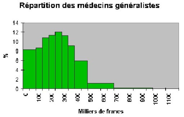
For this purpose we will represent the various classes of revenue on the X-axis and the percentage of physicians corresponding to each class on the Y-axis. If we are so careless as to brutally use the original table, we get the below chart.
We realise there is something terribly wrong with this chart: its scale does not allow a correct comparison across the classes.
In order to fix this, it is necessary to have the same amplitude (that is, the same interval width) for each class.
So we decide to use the smallest amplitude available from the original data as our base unit amplitude.
Note: Such choice is based on your objectives and usage for the data, another possible choice could consist in choosing the largest interval, if it better suits your purposes, then why not? Besides, each class should host enough individuals in order to interpret the height of the rectangle as an approximation the probability for the variable to belong to the class.
From the example the base unit amplitude will therefore be 50, which corresponds to the original interval of the classes [100;150[, [150;200[, [200;250[, [250;300[, and [350;400[.
These classes do not need our intervention as they already have our chosen unit as their interval. But we do need to modify the other classes that display a different interval.
E.g. the [500;700[ class. We know that 6.95% of the population belong to this class. And we need to split this class into classes of amplitude 50, i.e. [500;550[, [550;600[, [600;650[, and [650;700[.
Nothing in the data set can help us deciding on the counts of these four new classes.
We have arbitrarily decided to allocate evenly the count of the original class to the four new classes, thus giving 6.95% / 4 = 1.73% to each new class.
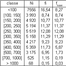
We will call this number corrected frequency, fi corr and modify the original table accordingly.
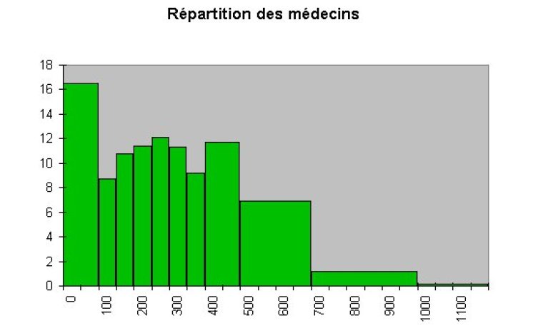
Eventually, we can draw a truly representative chart, called histogram.
The principle used here, equally works for discrete series representation.
Box Plot
The software packages you will use will flood you with numerous options destined to impress your audience with your subtle taste in graphical presentations. One of these options has been particularly successful: the box plot.
The box plot definition may slightly vary from software to software, always read carefully the software instructions.
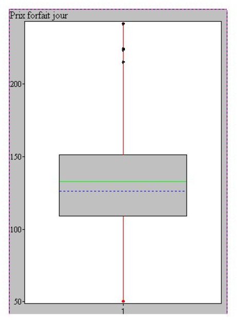
Here is the definition given by Spad.
For each box, the lower horizontal line represents the value of the first quartile (here 25%), the upper horizontal line represents the third quartile (here 75%).
The grey box thus represents 50% of the population.
The mean is represented by a full horizontal line and the median by a dashed horizontal line.
Up to where the vertical lines extend (French speakers refer to them as “moustaches”), is variable: {maximum/minimum}, {1st decile/9th decile}... check the definition of your favourite software.
The dots marked with black crosses are individuals with values considered “extreme” as defined by the TUKEY index i.e. 1.5 times the height of the grey box above (resp. below) the first (resp. third) quartile.
One of the advantages of box plots is to allow easy comparison of one population to another. In the following example, we observe the box plots for the price of ski passes in various regions of France.
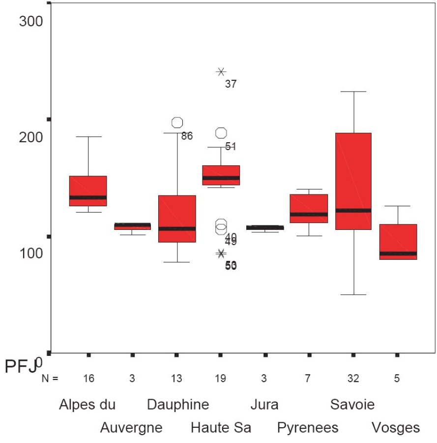
If we compare on this chart the price of ski passes in the regions of Savoie and Haute-Savoie, we find more homogenous and altogether higher prices in Haute-Savoie than in Savoie region .Did we just unveil anti-competitive practices? A Haute-Savoie cartel? Or is it something else? The data are statistical, the explanation remains yours.


